By: Mohamed Batran

LIDAR point cloud data is a collection of points that describe a surface or an object. Each point is described with x, y, z coordinates and in some cases is associated with additional attributes such as a classification of the point.

Often, LIDAR data is used to extract accurately georeferenced vector features such as buildings, roads, trees. To realize that there are two main steps as in [1]:

1. Classification: assign a class to each point in the point cloud dataset. One way is using the PointCNN neural network given that there is sufficient training data. The output is a class for each data point.
2. GIS pipeline: extracting relevant features from classified point cloud data in a usable format. In addition to extraction, generating attributes information to the extracted features such as object height, object surface area, centroid lat/lng, proximity to other features (e..g how far from the nearest road) and other.

This article will expand on point no (2) focusing on the GIS feature extraction assuming the data is already classified and each data point is assigned a class.

Data and Preprocessing

Data download and transformation

For sample data acquisition, one laz tile is downloaded from [3]. When working with geospatial data, it’s always important to know what is the spatial reference system of the dataset. The spatial reference system for this tile is EPSG:7415 [4].The definition of spatial reference system according to Wikipedia is

“A spatial reference system or coordinate reference system is a coordinate-based local, regional or global system used to locate geographical entities.”

The server to download the data is not very fast, so downloading may take some time. It took me a few hours to download the dataset. The downloaded file is in Laz format, that is a lossless compression of LIDAR data. It can compress original Las files to only 7 to 25 percent of their size. The speed is one to three millions points per second [5].

The downloaded file size is 2.2 GB. To decompress Laz files to the original Las one option is to use pylas. The extracted Las file is 13 GB. Impressive compression ratio! Below how to decompress a laz file to las file in python using pylas python package.

Point Cloud visual inspection

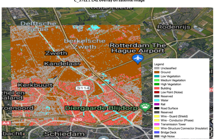
Starting from QGis 3.18, there is a feature to load and visualize las point cloud data. It’s pretty straightforward and allows data visualization, overlaying satellite imagery and rendering high quality maps. We had to manually define the CRS (Coordinate Reference System) of the point cloud file to appear on the viewer window of Qgis. For satellite imagery overlay, There are many qgis plugins, one of the best is Quick Map Services developed by next gis which have most known basemaps xyz urls [6]. The dataset we are using already has most points classified and can be mapped with a legend as below.

Looking closely at the classified point cloud with overlaid satellite images, we can see that not all features are exactly classified as in the background satellite image. Only Ground, Building, Water objects are captured and there is no additional information about e.g. Road surface of trees.

One reason may be that the date of point cloud data acquisition (2014) is different from the date of the overlaid background map (2021 by Google). Green areas are also misclassified as ground, maybe it was the winter season with a lot of snow?

For a Poc purpose, we should reduce the data size to the minimum AOI (Area of interest). However, we should also consider that the output algorithm on the minimum AOI will guarantee the same results when scaled to a bigger dataset. To do that, let’s hand pick an AOI that contain most of the classes and draw a polygon with the same CRS on the screen as below:

To clip LIDAR point cloud data to a specific AOI, there are many tools and libraries such as lastools clip or other python options such as PDAL. Why do we need to clip the LIDAR dataset into smaller area of interest:

1. In development phase, we need to tryout many solutions and running the script every time on a big dataset and waiting for the solution to validate is a nightmare
2. In most cases, development happens on local machines, where resources are limited. Then the same code can be used on cloud or a bigger server
3. It’s much easier to visually inspect the quality of the algorithm is the data size is small and can fit in memory.

The output smaller Area of Interest looks like this:

Quick visual investigation show that data contain classes of three categories:

1. Buildings
2. Ground
3. Water
4. Unclassified

Building features seem very well represented and have easy to identify geometrical shape. Water features look incomplete and will probably result in wired polygon pieces if we automate capturing it from this sample. For limiting the scope of this analysis, This work will focus on only Extracting buildings from the classified LIDAR data.

Feature extraction

According to [1] to extract objects from LIDAR data, There are two techniques to be used, each one of the two can be suitable for a specific use case and depending on the business requirement and acceptance criteria:

1. Raster analysis by rasterizing point cloud layers, then apply raster to polygon
2. Use unsupervised machine learning algorithm DBSCAN to separate each object as a cluster, then apply a bounding polygon operation or other to approximate the boundary of the object.

In this report, we will explain and apply both techniques.

(1)  Raster Analysis

To capture features from LIDAR data points, the first step is converting the 3d vector points (x,y,z) into grid-based raster representation. This process is called rasterization, the output raster will be a Digital Surface Model (DSM).  and will also contain the corresponding average points height in each pixel.

One library that can do that is Pdal  [7]. To move forward, we need to specify the resolution of the resulting DSM. In this case, let’s use 4 times the average spacing between points, this is best practice but can vary depending on the use case. The average spacing between points is roughly 30 cm ( manually measuring that on screen a few times), then we chose pixel size to be 1.2 meters.

To install pdal on mac, use the following command:

 Pdal has a python api to use in scripting and to create data pipelines from python, the api implementation is as below:

In the above code block, the JSON object pdal_json stores the required pipeline definition. First, we input the las file path as INPUT_LAS_PATH, Then we specify the limit class we want to extract is class no. 6, that is building. After that, we specify the output file name as OUTPUT_TIFF_DEM and the resolution of the output TIFF image.

Once we pass that definition document to pdal Pipeline api, it will start executing based on the input and output the TIFF file from the input last. Pretty straightforward and convenient.

This will result in a geotiff file as below, it’s a raster file with pixel size of 1.2 meter as we specified. Also each pixel contains the height of the pixel from the point cloud data. The visualization below can be generated using QGIS and quickmapservice plugin for background satellite images.

The next step is to extract the building footprint from the resulting DEM. There are more than one tool to do that. For e.g:

1. Using gdal polygonize implementation
2. Using rasterio shapes

Both tools create vector polygons for all connected regions of pixels in the raster sharing a common pixel value. Each polygon is created with an attribute indicating the pixel value of that polygon. Since the DEM contains the height of the pixel as a pixel value, extracting polygons from the dem file will result in multiple small polygons with the same pixel value. It’s not what we are looking for.

To extract building footprint, we should treat the dem as a binary tiff file where building pixels can be set to 1, and no building data are set to np.nan value. This preprocessing step can then feed into another process of rasterio shape extraction or gdal polygonize to extract pixels with the same value as one polygon.

Finally, having a polygonized coordinate set of each polygon. We can use shapely and geopandas to create a geo data frame with every building as a feature. Shapely and geopandas are one of the most famous geospatial data handling libraries in python.

Please note, In this step, the crs of the features should be set to 7415 before saving the output vector file . The total extracted features are 155 building

By doing that, we have iterated through each extracted polygon and saved them all to a list of geometres. Those geometries can be read in geopandas and will appear as geodataframe as bellow, with this, 90% of the hard work is completed.

The resulted vectorized building shapes look like below, later in this article we will apply a post processing step to extract meaningful features from those buildings, so keep reading. 

Unsupervised Dbscan clustering

In the previous section, we extracted the building footprint using raster analysis and polygonization. While this method works ok, it requires data transformation to a completely different type (Raster) which loses some important values associated with the original data points.

In the following method, we will use an unsupervised machine learning clustering method to cluster all points that are close to each other as one cluster, then extract building boundaries from those points.

LIDAR data is stored in a las file (or compressed laz file). To apply clustering, let’s first extract the coordinates of each point X, Y, Z and the associated class per point as below:

The resulting data format will be an array of points X, Y, Z, C where x is the longitude, y is the latitude, z is the elevation and c is the class of the point. Resulting total data points are 12,333,019 for the area of interest. To start with building data, let’s filter only the building class which is class no. 6. This result in a total number of 1,992,715 building points

The points above can then be visualized on a background map to view how building classes look like in 2d, in this case each data point is stored as a 2d gis point stored in a shape file and elevation is an attribute. Which is different from the las file data storage before. 

The next step after that is applying 3d clustering using DB scan. DB scan is Density-Based Spatial Clustering of Applications with Noise. Finds core samples of high density and expands clusters from them. Good for data which contains clusters of similar density.

In DB scan, there are two core parameters, first one is epsilon which is The maximum distance between two samples for one to be considered as in the neighborhood of the other. The second parameter is min_samples, that is the number of samples (or total weight) in a neighborhood for a point to be considered as a core point. This includes the point itself.

Using DB SCAN algorithm, the output is as follows where every point is associated a cluster label that separate that cluster from other data points, for points that are noise and not close to other points within the epsilon parameter, the algorithm will set it’s value to -1 as it is not associated to any cluster data point. See how clear the output is?

The next step is using data points of each cluster to extract the building footprint and the associated attributes of this object. In order to process each cluster individually, the problem statement is as follows:

Given an object 3d coordinates:

1. Extract the mean elevation of that object
2. Calculate the 2d boundary of the object
3. Calculate the associated geometry details such as area and centroid point.

The total number of points in the above building = 35580 point

Let’s take some time to look how clean the borders are based on the input points.

For every building, we are able to compute the following attributes while is very useful for using the output data file:

1. Boundary geometry
2. Elevation of the building by taking the median altitude of points
3. Total Area
4. Perimeter
5. Centroid x coordinates
6. Centroid y coordinates

To interactively look at the resulted 3d building shapes, click here: 

Post processing

It’s common to apply post processing after the main processing pipeline is completed. The purpose of the post processing work vary from one project and data type to another, broadly speaking those are some post processing target objectives:

1. Quality check and outlier removal

For example, removing features with unrealistic area or with small area, detecting overlapping features and merging them, and so on

1. Geometrical calculation

For example, calculating features centroid, calculating feature

1. Enrichment

Adding more attribute information to features from external dataset, e.g. attaching distance of all houses from the nearest bus stop by referring to an external data source of bus stops.

Quality check and outlier removal

Automating quality check and outlier removal need a fairly good understanding of the permitted applications of the extracted features and collaboration with end users or the product manager (the end user’s voice) to put together a final product quality acceptance criteria.

For our use case, we will limit the scope of quality check and outlier removal to the area of the extracted building where it should be within a reasonable range. For this purpose, we will assume that the smallest building consist of one room 3*3 square meters (9 square meters). This post preprocessing step will eliminate 40 polygons leaving the total extracted buildings in the area of interest to 115.

Geometrical calculation

For practical business use, and to create an easy to query dataset, meaningful calculated attributes for each feature can be extracted in the post processing step. An example of those features are area, centroid x, centroid y to name a few. This step will later help non geospatial data users to query the data for various business use cases and utilization.

Geometry calculation is pretty straight forward in geopandas as below

Data enrichment

Enrichment commonly refers to appending or otherwise enhancing collected data with relevant context obtained from additional sources. Geospatial data enrichment means adding more attributes to the dataset by referring to external data sources. Few common data sources are:

1. Road infrastructure networks
2. POI database
3. Demographics distribution
4. Administrative boundaries

We will skip applying this step in this report.

Engineering

1.   Code formatting 

Using Yapf [8] by google to style the output code

yapf building_extractor.py > building_extractor_styled.py

2.   Dockerization

It’s a good practice to dockerize a python application to avoid dependencies conflicts, especially in this case we used so many libraries and some of them rely on binary data that are separately installed such as PDAL. Reproducing the same environment without docker will be challenging

3.   Unit tests

Logical functions such as alphashape algorithm, geometry calculation should be tested using unit tests before running the output.

Summary

LIDAR data processing is essential for many applications such as mapping and autonomous driving. For most applications, automating object detection and extraction is necessary to ensure the business success of a LIDAR product. While a lot of tools now offer out of the box analytics such as Arcgis, programming one’s own tools give more flexibility to add or adjust to a specific use case. In this article we explored how to extract building footprint from LIDAR dense point cloud using two different techniques:

1. Rasterization and polygonization
2. Unsupervised machine learning density based clustering and alphashape boundary detection

We also explored the standard post processing techniques such as

1. Geometric calculation to extract essential properties about each geometry such as area, perimeter and centroid
2. Enrichment to append more entity attributes from external datasets such as road network of POIs database if needed

Finally, we looked into some engineering steps to ensure code reusability such as:

1. Code formatting using automatic formatting tool
2. Dockerization
3. Unit testing

The whole analysis in this report can be automated end to end and scheduled as a batch job if needed.

References

[1] https://medium.com/geoai/object-extraction-from-mobile-lidar-point-clouds-with-machine-learning-cb15fcbb5597

[2] https://github.com/beedotkiran/Lidar_For_AD_references

[3] https://download.pdok.nl/rws/ahn3/v1_0/laz/C_37EZ1.LAZ 

[4] https://epsg.io/7415

[5] https://www.cs.unc.edu/~isenburg/lastools/download/laszip.pdf

[6] https://plugins.qgis.org/plugins/quick_map_services/

[7] https://github.com/LAStools/LAStools

[8] https://pdal.io/workshop/exercises/analysis/dtm/dtm.html

[8] https://github.com/google/yap